
 Abosh
Cp compares a process’s six-sigma spread with the width between specification limits. Cpk also accounts for how close the process mean is to the nearest limit. Calculate these indices only with a suitable, stable process model and a clearly defined estimate of variation. A high Cp with lower Cpk points to an off-centre process. Neither index by itself proves long-term quality, measurement accuracy or compliance with a customer’s acceptance rules.
Calculate Cp and Cpk from declared millimetre inputs.
Separate centring problems from excessive variation.
Know when a capability number is not trustworthy.
Start with specifications, not control limits
A drawing or customer agreement sets specification limits. Statistical control limits describe how the process has behaved. Moving one to resemble the other changes the question rather than fixing the process.
NIST frames capability as a comparison between a stable process and its specifications. First check the measurement system and time-ordered data. A calculation across tool changes, materials or unexplained shifts can hide several different processes inside one standard deviation.
This guide answers the capability calculation. Control charts address stability; Gage R&R addresses measurement variation.
Two indices, two practical questions
Let USL and LSL be the upper and lower specification limits, μ the process mean, and σ the standard deviation used to describe within-process variation. Keep all three dimensional quantities in the same unit.
Cp asks whether the spread could fit between the limits if centred. Cpk uses the smaller distance from the mean to either limit. A mean outside a limit produces a negative side index; do not hide that result by taking an absolute value.
Cpk = min[(USL − μ)/(3σ), (μ − LSL)/(3σ)]. State how sigma was estimated and why the process model is appropriate.
A shaft that drifts toward the upper limit
Illustrative example: a shaft diameter has limits of 9.90 and 10.10 mm. A suitable within-process estimate gives σ = 0.025 mm. The six-sigma spread is 0.150 mm, compared with a 0.200 mm specification width.
At a mean of 10.00 mm, each limit is 0.100 mm away. Cp and Cpk both equal 1.333 before rounding. If the mean moves to 10.04 mm while σ remains unchanged, the upper distance falls to 0.060 mm. Cpk becomes 0.060 / 0.075 = 0.80.
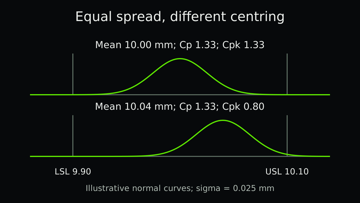
| Teaching scenario | Mean | Cp | Cpk |
|---|---|---|---|
| Centred | 10.00 mm | 1.33 | 1.33 |
| Shifted upward | 10.04 mm | 1.33 | 0.80 |
Try the Cp and Cpk calculation
Change the mean while keeping sigma fixed, then change sigma. Use one unit throughout. These are supplied inputs, not estimates from raw measurements.
- Cp
- 1.333
- Cpk
- 0.8
Calculations stay in your browser. Inputs are not saved after leaving this page. Download the record if you need to keep it.
Keep the estimate behind sigma
Use the calculator to check the arithmetic, not to certify a process. Record the measurement method, sample period, subgroup design and within-process estimator beside your result. An overall standard deviation may answer a different question and is often reported with Pp/Ppk.
A negative Cpk is possible when the mean crosses a specification. Zero sigma does not establish infinite capability; it can reflect rounding or inadequate measurement resolution. The calculator leaves that case undefined.
Choose and disclose the variation estimate
A capability report should identify subgrouping, sample size, period and estimator. Within-subgroup variation and overall variation can differ when the process drifts. Software often labels overall indices Pp and Ppk; check its definitions rather than assuming every report uses the same sigma.
The conventional formulas assume a suitable distribution, commonly normal, and representative observations. Strong skew, mixtures or autocorrelation need a justified alternative analysis. An automated normality checkbox cannot establish that the sample represents future production.
- Verify the measurement process
Check resolution, calibration, repeatability and the operators or instruments represented.
- Check time-ordered behaviour
Investigate special causes before estimating a stable-process capability. Keep different conditions separate when necessary.
- Calculate with traceable inputs
Record limits, units, mean, sigma method, sample size and date range. Retain unrounded values.
- Compare with the actual requirement
Use the applicable customer or internal acceptance rule and appropriate uncertainty, not an unexplained universal cutoff.
Cpk vs Ppk: use the same record
Cpk uses a declared within-process variation estimate. Ppk conventionally uses overall variation across the observation period. Both use the same mean and specifications here. Neither name guarantees a short-term or long-term study: record the actual period and conditions. Minitab’s comparison explains why drifting subgroup means can make the two results differ.
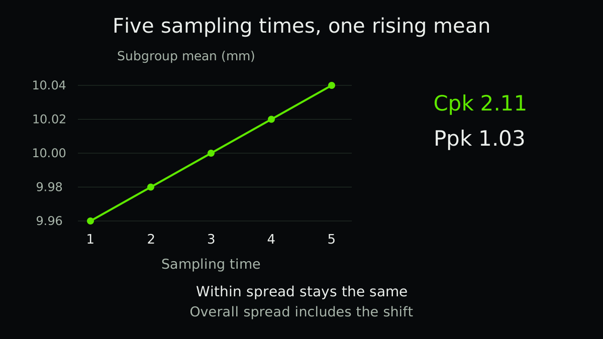
Fictional teaching record: take five consecutive parts at each of five successive sampling times, measured in mm. The subgroup means rise from 9.96 to 10.04. This deliberately arranged drift makes the example unsuitable for claiming a stable capability or a future defect rate. Twenty-five readings also make a poor qualification study.
| Sampling time | Five consecutive readings (mm) | Mean (mm) |
|---|---|---|
| 1 | 9.94 / 9.95 / 9.96 / 9.97 / 9.98 | 9.96 |
| 2 | 9.96 / 9.97 / 9.98 / 9.99 / 10.00 | 9.98 |
| 3 | 9.98 / 9.99 / 10.00 / 10.01 / 10.02 | 10.00 |
| 4 | 10.00 / 10.01 / 10.02 / 10.03 / 10.04 | 10.02 |
| 5 | 10.02 / 10.03 / 10.04 / 10.05 / 10.06 | 10.04 |
Recalculate the two variation estimates
The grand mean is 10.000 mm. For this example, pool squared deviations from each subgroup’s own mean, divide by 5 × (5 − 1) = 20, then take the square root. No unbiasing correction is applied. The within sum of squares is 0.005000 mm², giving 0.015811 mm. Other estimators or correction settings can give different answers; Minitab documents those options.
For overall sample standard deviation, use deviations of all 25 readings from the grand mean. Their squared deviations sum to 0.025000 mm². Divide by 25 − 1 = 24 and take the square root: 0.032275 mm. With limits 9.90 and 10.10 mm, the nearest limit is 0.100 mm away. Cpk is 0.100 / (3 × 0.015811) = 2.11; Ppk is 0.100 / (3 × 0.032275) = 1.03. Calculate with unrounded inputs.
The gap points to variation between sampling times that the within estimate leaves out. Plot the readings in time order and investigate subgroup formation, measurement changes, offsets and temperature. Do not remove inconvenient groups just to raise Ppk. In real studies, use enough representative subgroups and suitable control-chart analysis before interpreting capability.
sp² = ΣiΣj(xij − x̄i)² / Σi(ni − 1); s² = Σij(xij − x̄)² / (N − 1). All measurements use mm.
| Variation estimate | Standard deviation (mm) | Nearest-limit index |
|---|---|---|
| Within, pooled; no bias correction | 0.015811 | Cpk 2.11 |
| Overall, sample SD | 0.032275 | Ppk 1.03 |
Do not turn 1.33 into a universal pass mark
Some contracts specify index thresholds. Others require particular sampling, confidence, measurement studies or methods for non-normal data. Follow the requirement for this characteristic and application.
An estimated Cpk is uncertain, especially from a small sample. NIST discusses confidence limits for capability indices. A point estimate just above a contractual boundary can be much less reassuring than the displayed decimals suggest.
A capable historical sample also cannot prove tomorrow’s output will stay acceptable. Continue monitoring the process and confirm actual first-pass yield.
What do Cpk 1.33 and 1.67 mean in sigma units?
For the conventional formula above, the mean-to-nearest-specification distance is 3 × Cpk × the stated within-process sigma estimate. Cpk 1.33 therefore corresponds to about 3.99 such sigma units; 1.67 corresponds to about 5.01. These are rounded index interpretations, not guarantees of a particular defect rate.
The interpretation needs a stable process, suitable measurement data and an appropriate distribution and variation estimate. If the mean lies outside a specification, Cpk can be negative. Do not take an absolute value or call that a safe positive distance.
An assumed 1.5-sigma long-term shift is a separate convention, not part of the Cpk formula. State any shift assumption explicitly rather than converting every Cpk result into a Six Sigma level. NIST's capability guidance describes the indices and their assumptions; release decisions also need the applicable customer requirements.
With no assumed mean shift and the same sigma definition, a nearest limit four sigma units away gives Cpk = 4/3, about 1.33. A nearest limit six sigma units away gives Cpk = 6/3 = 2.00. These algebraic relationships do not establish that a drifting process will maintain those distances over time.
Keep capability connected to a decision
For a stable but off-centre process, a documented centring investigation may help. For excessive spread, focus on the sources of variation. If the process is unstable, resolve that instability before advertising a capability number.
Use capability alongside inspection results, failure consequences and sampling coverage. Predictive quality adds another evidence layer, but a model score cannot repair misleading measurement inputs.
What would Cpk 0.67 mean?
Using the conventional formula and the same stated within-process sigma estimate, the nearest specification is 3×0.67 =2.01 such sigma units from the mean. That is a conditional interpretation of the index. It is not an observed reject percentage or a guarantee about future production.
Check stability, measurement quality, subgroup design, distribution assumptions and the actual acceptance requirement before deciding what to do. A rounded 0.67 cannot diagnose whether the problem is centring, spread, mixed conditions or an unsuitable estimator. Keep the time-ordered observations with the calculation.
A related example from Abolfazl
Compare the capability formulas and their assumptions in another worked example.
In English, on founder Abolfazl’s personal blog. This is related reading, not an independent technical source.
Practical checklist
- Confirm the current specification revision.
- Keep units consistent.
- Check the measurement system.
- Inspect time order and process stability.
- State the distribution and sigma estimator.
- Separate materially different production conditions.
- Record sample size and estimation uncertainty.
- Apply the actual acceptance agreement and keep monitoring.
FAQ
FAQ
Sources and further reading
Authoritative references used to research and verify this guide.